4.0 What the ORS delivers, and why the weighting is asymmetric
The Operational Readiness Score measures how sale-ready a chain is from the inside. Five sub-components decompose that readiness into orthogonal dimensions, each with its own formula, its own bandwidth, and its own data path. An operator can stand the ORS up for their own chain inside a single quarter, provided consolidation reporting delivers unit-level data. Where it does not, this section documents the approximations that remain admissible.
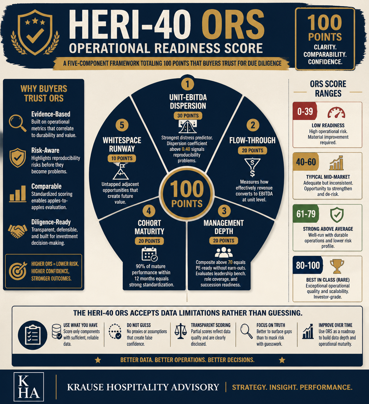
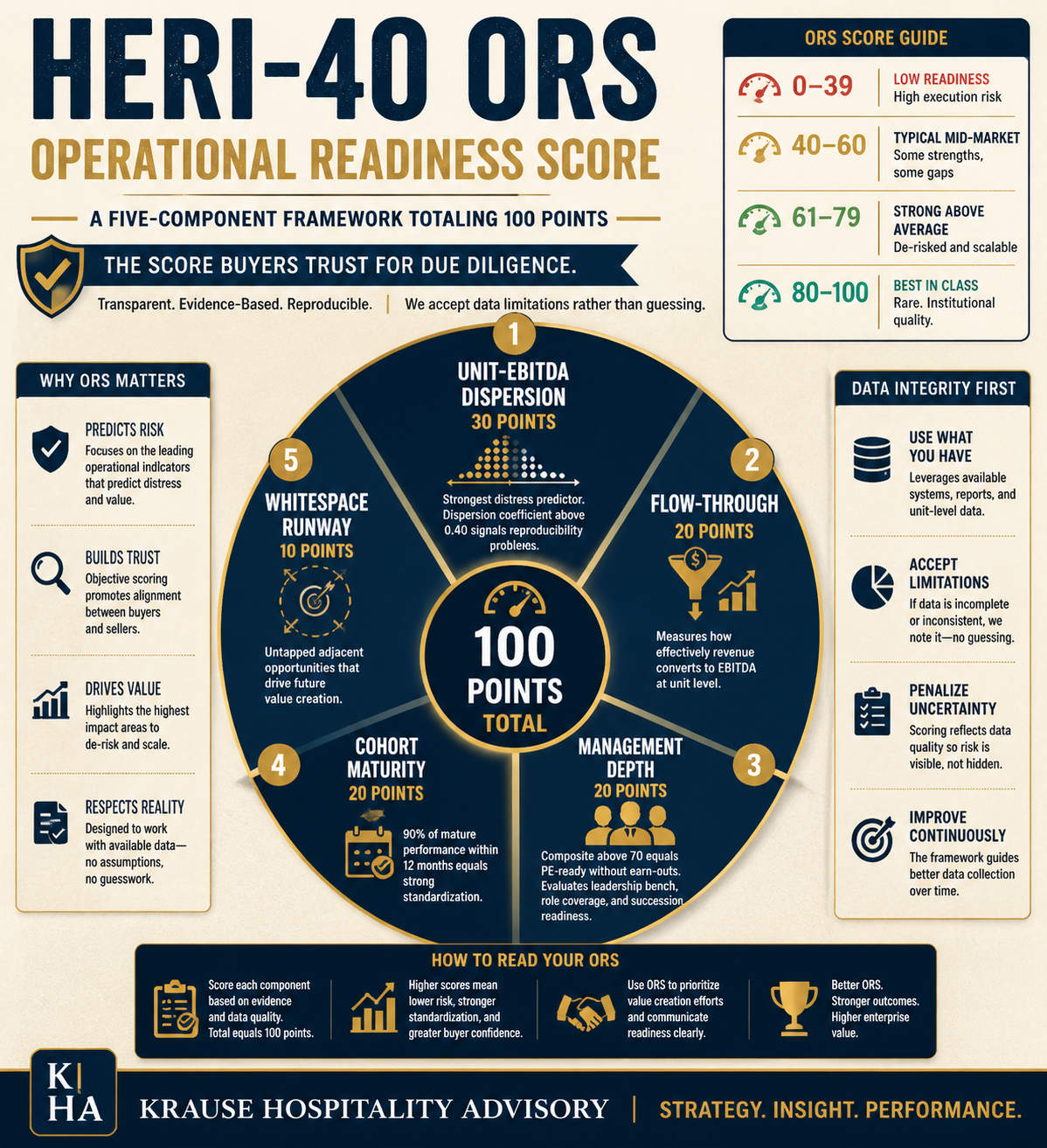
Five components, not three and not eight. That number is the output of the retrograde backtest in Appendix A: each sub-component addresses a separate buyer objection that proved to be valuation-relevant in the documented hospitality deals from 2018 to 2025. Flow-Through (A1) shows whether the business model scales. Unit-EBITDA dispersion (A2) shows whether the scaling is reproducible. Management depth (A3) shows whether the system survives without the founder. Cohort maturity (A4) shows whether new locations reach the mature-store level on a predictable timeline. Whitespace runway (A5) shows whether enough growth distance remains to compose an attractive buyer target picture. Fewer components would leave blind spots in the valuation. More components would dilute the reading and strip the methodology of its edge.
The weighting is not evenly distributed. A2 (unit-EBITDA dispersion) carries 30 of 100 points; A5 (whitespace runway) only 10; the remaining three 20 apiece. That asymmetry is not intuitive and it is not arbitrary. Both cross-check passes of the backtest arrived independently at the same result: unit-EBITDA dispersion was, in every documented distressed case, the earliest and strongest indicator of the later value correction. A chain that showed, in quarter X, a dispersion above the critical threshold was, in the documented cases, 18 to 24 months later either in value correction or in restructuring. Whitespace runway, by contrast, is the most speculative of the five components, because its computation rests on modelled assumptions about competitive density and cannibalisation that are, in sale processes, frequently interpreted in the seller's favour. Hence the lighter weight. Appendix A documents the backtest logic in detail.
In the following five subsections we decompose A1 through A5 in sequence. Each subsection contains formula, calculation path, DACH bandwidth, data sourcing, interpretation zones, and a score-mapping table. To avoid tracking the methodology in the abstract, we carry an anonymised example operator through all five components: a premium-casual DACH operator with 47 locations, seven years of system maturity, and a capital-round sounding inside the next twelve months. We refer to this operator as XY. At the end of Section 4.6 we sum its five sub-scores into a total ORS.
4.1 A1 — Flow-Through % (weight 20 points)
4.1.1 What Flow-Through measures
Flow-Through is the percentage of each additional unit of revenue that reaches the bottom line as an additional unit of EBITDA. Through a PE lens, Flow-Through is the single most important proof of operating leverage: it shows that the cost structure is scalable, without requiring the hand-over of unit-level P&L data to a prospective buyer. If each additional unit of revenue yields 30 cents of additional EBITDA margin, the cost curve is flat. If each additional unit yields only 10 cents, the curve is convex. Convex cost curves are problematic in scaling, because they systematically hold EBITDA margins below the sector standard.
In the retrograde backtest against the ten documented hospitality deals 2018 to 2025, Flow-Through turned out to be the earliest distressed early-warning signal: in every insolvency case, a declining Flow-Through trend was already visible across several quarters before the wave of location closures began. Buyers who track Flow-Through as a quarterly metric would have had 12 to 18 months of lead time in every documented case.
4.1.2 Formula and calculation path
The formula is a delta calculation across four rolling quarters, with the same unit set in numerator and denominator. The same unit set is decisive: mixing location openings or closures into the calculation no longer measures operating leverage — it measures portfolio-mix effects.
Formula: Flow-Through % = (Unit-EBITDA Quarter Q − Unit-EBITDA Quarter Q−4) / (Unit-Revenue Quarter Q − Unit-Revenue Quarter Q−4).
Two worked examples for illustration. A 50-location chain with a constant unit set across four quarters: unit revenue rose by EUR 1.2 million, unit EBITDA by EUR 380k. Flow-Through 380k / 1.2m = 31.7%. A solid value for a fast-casual chain, pointing to a mature cost structure. Second case, same size: unit revenue rose by EUR 1.8 million, unit EBITDA by only EUR 220k. Flow-Through 220k / 1.8m = 12.2%. The additional revenue unit was consumed almost 90% by additional cost. This signals a structural cost-structure problem that must be addressed before any sale conversation.
4.1.3 Bandwidth by segment
Flow-Through expectations differ by segment because the underlying cost structures differ. QSR with high automation and supply-chain standardisation typically reaches higher values than full-service with a higher labour share.
- QSR: 25% to 35% counts as healthy, above 35% as exceptional.
- Fast-casual: 20% to 30% healthy; the corridor is narrower than in QSR.
- Full-service restaurant (FSR): 15% to 25% healthy, because labour cost scales more steeply with growth.
- Below 15% across several quarters signals a cost-structure problem in every segment.
- Above 40% is explicable only where a one-off cost lever was pulled (energy hedge, labour restructuring, raw-material lock-in). Such values rarely persist for two quarters.
Premium-casual operators sit between fast-casual and FSR; depending on labour intensity, the realistic corridor is 17% to 25%.
4.1.4 Data sourcing
The clean source is the quarterly unit P&L drawn from the ERP. Where consolidation reporting runs at location level, the value is directly derivable. Where only aggregated quarterly reports are available, two approximation paths deliver a defensible value.
For franchise systems that consolidate royalty and marketing-fund reporting, Flow-Through can be approximated from prime cost (cost of goods plus labour as a share of revenue) plus royalty plus estimated location rent and location labour. This approximation has an accuracy margin of roughly three percentage points — sufficient for trend statements, borderline for point estimates.
For listed peers in the sub-segment, Flow-Through can be approximated from segment reporting in the quarterly filings. Caution applies here too: consolidated group reports smooth out effects that would be visible at unit level.
Where unit EBITDA is not directly available, the approximation via EBITDAR minus estimated rent is admissible, provided the assumption is transparent in the buyer conversation. Buyers accept approximations when the methodological path is documented. They do not accept approximations sold as precision.
4.1.5 Interpretation zones and typical pitfalls
Five zones for placing your Flow-Through value:
- Below 15%: structural cost problem. Address before any sale conversation.
- 15% to 20%: acceptable, but below the level premium buyers expect.
- 20% to 30%: healthy. The corridor in which most mature hospitality operators sit.
- 30% to 40%: strong. Operating leverage as a defensible sale argument.
- Above 40%: exceptional. Explicable only via one-off effects or an atypically flat cost structure.
Three pitfalls regularly distort Flow-Through values. First: energy hedges and commodity spikes can shift a single quarter's value by five to ten percentage points without any change to the cost structure. Recommendation: flag one-quarter outliers rather than smooth them — buyers will ask anyway. Second: seasonality mix shifts values when the calculation is not run strictly rolling across four quarters. Third: extraordinary marketing spend during opening phases depresses Flow-Through but belongs to normal investment logic. Here the separation between growth marketing and run-rate operations marketing matters.
4.1.6 Score allocation 0–20 points
| Flow-Through % | Score |
|---|---|
| Below 10% | 0 |
| 10% to 15% | 5 |
| 15% to 20% | 10 |
| 20% to 30% | 15 |
| Above 30% | 20 |
Example operator XY: premium-casual operator with 47 locations, seven years of system maturity. Trailing-four-quarter calculation across the same 38-location set (nine locations opened only after the cut-off date, therefore excluded): unit revenue rose by EUR 4.1 million, unit EBITDA by EUR 740k. Flow-Through 18.0%. Placed inside the premium-casual bandwidth (17% to 25%): at the lower edge of the healthy corridor, not alarming but not a premium argument either. A1 score: 10 points.
4.2 A2 — Unit-EBITDA dispersion (weight 30 points)
4.2.1 Why A2 is the single most important signal
Unit-EBITDA dispersion is the only metric in the ORS that answers the question "Is your system reproducible?" directly. Operating leverage (A1) shows whether the business model scales. Dispersion shows whether the scaling succeeds equally at every unit. The distinction is decisive in the buyer conversation: a chain with high A1 but broad dispersion sells, at its core, founder genius that does not transfer to new locations. A chain with moderate A1 and tight dispersion sells a systemic playbook that institutional buyers accept as a valuation basis.
The cross-check validation from the retrograde backtest warrants attention. Both independent backtest runs identified A2 as the sub-component with the highest predictive power for later distressed developments. In every documented insolvency case, unit-EBITDA dispersion sat above the critical threshold 18 to 36 months before the insolvency. In no premium-multiple deal did it sit above that threshold. The signal strength is asymmetric relative to the four other components — hence the weighting at 30 rather than 20 points.
The methodological implication: if you have time for only one ORS sub-component, compute A2. Where your A2 reading sits above 0.40, the discussion of the remaining components is secondary — you have a playbook reproducibility problem that must be addressed before any sale conversation.
4.2.2 IQR normalisation: why IQR divided by median
The formula is the interquartile range of unit-EBITDA values, divided by the median. IQR rather than standard deviation, because a single loss-making location would dominate the standard deviation — whereas the target is to measure the typical dispersion of the majority of locations, not the effect of an outlier. Division by median rather than mean, because extreme values distort the mean in small samples but not the median.
A worked example for clarity. A chain of 40 locations, sorted by unit EBITDA: the location at the 25th percentile (P25) generates EUR 100k of EBITDA, the median (P50) sits at EUR 150k, the 75th percentile (P75) at EUR 210k. The interquartile range IQR is the difference P75 minus P25, i.e. EUR 110k. Divided by the median: 110 / 150 = 0.73. A dispersion of 0.73 is high and sits outside the corridor of a reproducible playbook. In the reading of the bandwidth below, this chain is a case that requires explanation.
4.2.3 Bandwidth and interpretation
Four zones for placing unit-EBITDA dispersion:
- Below 0.25: reproducible playbook. Your locations operate inside a tight corridor — an institutional buyer accepts the system as an investment basis.
- 0.25 to 0.40: acceptable. Some locations over- or underperform, but the typical unit sits close to the median.
- 0.40 to 0.60: requires explanation. Dispersion at this level will prompt due-diligence questions that must be answered with concrete location-level plans.
- Above 0.60: systemic playbook risk. In the documented backtest cases, this was the zone in which distressed developments originated.
Two publicly traceable reference values emerge from the backtest. Wingstop and Jersey Mike's sit, by evaluation of their FDD Item 19 dispersion data, below 0.30. Vapiano in its quarterly reports 2018 to 2020 sat above 0.60, with a rising trend up to the insolvency in spring 2020. The dispersion trajectory was publicly traceable; it was read in the market commentary of the time as a concept crisis, not as an operative reproducibility problem. The HERI-40 frame would have named the signal earlier and more sharply.
4.2.4 Data sourcing — the DACH gap
In the US market, FDD Item 19 provides a standardised disclosure format that makes unit-level EBITDA dispersion publicly traceable for many franchise systems. In DACH there is no equivalent. That is a real data gap which, as an operator, you close for the A2 calculation via one of three paths.
First, the clean path: from internal consolidation reporting at unit level. If the ERP outputs quarterly EBITDA per location, IQR and median can be computed directly. Sample size should be at least 20 locations with twelve months of trailing data each, otherwise noise dominates.
Second, the approximation via revenue percentiles: where only location revenue is reliably tracked, multiply the revenue percentiles by segment-typical EBITDA margins (QSR 18% to 22%, fast-casual 14% to 18%, FSR 10% to 14%, premium-casual 12% to 17%) and compute the approximated EBITDA distribution. Accuracy roughly five percentage points. Buyers accept this approximation if the margin assumption is transparently documented and not presented as precision.
Third, extrapolation from a location-audit sample: for smaller chains or for operators without consolidation reporting, a sample of at least 20% of locations can be audited at Q4 P&L depth and the result extrapolated to the full portfolio. The method is labour-intensive but, for mid-sized operators, often the only defensible option.
Where none of these paths is viable, A2 should not be guessed. Leave the component open, document the data gap, and use a reduced ORS score on a 70-point basis rather than 100. Buyers accept "not computed because data basis is missing" — they do not accept guessed values that due diligence later disproves.
4.2.5 Benchmarks by chain maturity
An A2 reading without a maturity frame is misleading. Young systems structurally carry wider dispersion than mature ones, because new locations are still on the maturation trajectory. Expected values by maturity:
- System age below 5 years: 0.40 to 0.60 typical. A chain at this age sitting at 0.30 is excellent.
- System age 5 to 10 years: 0.25 to 0.45 typical. Dispersion should decline continuously here.
- System age above 10 years: 0.15 to 0.30 typical. Values above 0.40 at this maturity are alarming because they point to structural reproducibility problems that do not dissolve with further scale.
The implication for self-diagnosis: A2 read in isolation carries less signal than A2 read inside the maturity context. An operator with eight years of system maturity and A2 of 0.32 sits inside the expected corridor; the same value at a 15-year chain would be grounds for structural review.
4.2.6 Score allocation 0–30 points
| Unit-EBITDA dispersion | Score |
|---|---|
| Above 0.60 | 0 |
| 0.45 to 0.60 | 10 |
| 0.35 to 0.45 | 15 |
| 0.25 to 0.35 | 20 |
| 0.20 to 0.25 | 25 |
| Below 0.20 | 30 |
An A2 score above 25 points is the strongest single signal of exit readiness in the entire methodology. Scoring 25 or more points here delivers, independent of the remaining ORS components, the sharpest reproducibility proof an institutional buyer accepts.
Example operator XY: seven years of system maturity, premium-casual, 47 locations. Calculation from internal reporting: median unit EBITDA EUR 165k, P25 at EUR 125k, P75 at EUR 215k. IQR EUR 90k divided by median EUR 165k yields dispersion 0.55. In the maturity context (seven years): at the upper edge of the expected corridor, more dispersion than desirable for a mature system. In the backtest comparison the value sits in the "requires explanation" zone. A2 score: 10 points. Corrective action: in the buyer conversation, dispersion is explained as the deliberate consequence of a location-mix strategy (two deviating location formats running in parallel), and the value is reduced to 0.40 across the next 18 months. That outcome yields an additional five to ten A2 points.
4.2.7 A warning against cherry-picking
Operators who "optimise" A2 ahead of a sale process by closing or carving out weak locations will have the historical dispersion trajectory placed on the due-diligence table. Buyers routinely request IQR/median rolled across three years, with explicit reference to location closures inside the same window. A cleaned A2 that drops from 0.55 to 0.30 without a cleanup disclosure will be recognised as a cleanup effect and devalue the signal.
The right sequence: cleanups only with adequate lead time, at least 18 to 24 months ahead of the sale process. The closed locations then fall out of the rolling three-year view, and the dispersion improvement is read as operating performance rather than a seller manoeuvre.
4.3 A3 — Management depth (weight 20 points)
4.3.1 Why management depth matters
Institutional-scale buyers ask the same question before every letter of intent: what does it cost to replace the founder in three years? If the answer is "the chain runs without him", the negotiation is about multiples. If the answer is "the chain rises and falls with him", the negotiation is about earn-out structures, non-compete covenants, and multi-year management contracts with lock-in clauses. In the worst case, there is no further negotiation at all, because the buyer classifies key-person risk as non-absorbable.
A3 measures the answer to that question as a reproducible number. The point is not that a founder wants to be replaceable — the point is that the buyer system can classify a founder as replaceable. That two-perspective distinction is decisive in the sale conversation.
4.3.2 The four scoring components
Management depth is computed as a weighted composite score on a 0-to-100 scale, drawn from four sub-components:
Component A — operating decisions without founder or C-level involvement (0–40 points). What share of daily operations decisions runs without escalation to the founder or the C-level? In scope: procurement (supplier selection and terms), personnel (hiring of location management and shift management), location operations (marketing actions, menu adjustments, pricing). Complete operating independence of location management in all three areas yields 40 points; complete founder escalation in at least one area yields 0 points. Most operators sit in the 20-to-30 corridor, because either procurement or personnel decisions are still centrally controlled.
Component B — C-level staffing COO/CFO/CTO (0–30 points). Are COO, CFO, and CTO professionally staffed — meaning with experienced external executives, not with founder-family members or the founder themselves in a double role? Full staffing of all three positions yields 30 points. Two staffed, one not: 20 points. One staffed: 10 points. None: 0 points. Buyers accept external interim appointments in this count when documented for at least twelve months.
Component C — middle-management retention 24 months (0–20 points). What is the turnover rate in the middle management layer across the last 24 months? The middle management layer encompasses location managers and area managers. Turnover below 15% per year: 20 points. 15% to 25%: 10 points. Above 25%: 0 points. This component is hard-measurable and verified in the buyer conversation through personnel records.
Component D — succession plan documentation (0–10 points). Is there a written succession plan for key positions, is it current (updated in the last twelve months), and has the board or shareholder meeting seen and minuted it? All three criteria satisfied: 10 points. Written but older than twelve months or not board-minuted: 5 points. Nothing documented: 0 points.
The sum of the four components yields a composite score on the 0-to-100 scale, which is translated into the ORS score through the mapping table in 4.3.6.
4.3.3 Self-scoring guidance
For most operators the calculation takes 30 to 45 minutes, provided the data basis exists. Example for a 47-location chain:
- Component A: location managers decide procurement up to EUR 5k single-ticket (regional suppliers) themselves, personnel up to shift-manager level themselves, marketing actions only within a pre-set frame. 26 of 40 points.
- Component B: COO externally staffed for three years, CFO externally staffed for 18 months, CTO position vacant. 20 of 30 points.
- Component C: middle management at 18% turnover across the last 24 months. 12 of 20 points.
- Component D: succession plan written, drafted 14 months ago, not board-minuted. 4 of 10 points.
Composite sum: 26 + 20 + 12 + 4 = 62 of 100 points. Placement in the bandwidth (see 4.3.4): earn-out required, but no deal-killer.
4.3.4 Interpretation zones
- Above 70 composite points: PE-ready without earn-out. Buyers accept the takeover without multi-year lock-in of the founder.
- 50 to 70 composite points: earn-out required. Typical lock-in duration 18 to 36 months, with performance-linked tranches.
- Below 50 composite points: key-person risk as deal-killer. Operators in this zone should defer the sale process and build management depth deliberately.
4.3.5 Subjectivity disclaimer
Components A and D contain judgement shares that can vary between assessors. Component A measures "share without escalation" — what the founder perceives as a routine decision, the COO may record as an escalation point. Component D evaluates "currency" and "board minuting" — again, judgement latitude applies.
The robust methodology is consensus scoring by three independent assessors: founder, COO, and an external advisor (M&A banker, board member, or coach). Each completes the matrix independently, then the median per component is taken as the consensus value. This method typically reduces deviation to under eight composite points.
In buyer verification, Component A is audited through interviews with location and area managers; Component D through presentation of the document and the board minutes. Optimistic self-assessments are systematically corrected in this phase.
4.3.6 Score allocation 0–20 points
| Composite score | Score |
|---|---|
| Below 30 | 0 |
| 30 to 50 | 5 |
| 50 to 65 | 10 |
| 65 to 80 | 15 |
| Above 80 | 20 |
Example operator XY: composite sum 62 of 100, computed as in 4.3.3. Sits in the "earn-out required" zone. A3 score: 10 points. Path to improvement: a CTO appointment inside the next 12 months lifts Component B by 10 points; a board-minuted succession-plan update lifts Component D by 5 points. That would move the composite to 77 and the A3 score to 15 points, and reduce the earn-out requirement substantially in the sale negotiations.
4.4 A4 — Cohort maturity (weight 20 points)
4.4.1 What cohort maturity delivers
Cohort maturity is the proof that the roll-out is reproducible. Where A2 measures the dispersion of mature locations, A4 measures the learning speed of new locations: how quickly does a 2024 opening cohort reach the level of the 2018 mature stores? The shorter the trajectory, the higher the reproducibility of the opening playbook, and the more attractive the chain to institutional buyers who intend to open further locations in the first 18 to 36 months after takeover.
Through a PE lens, A4 is the most important forward-looking signal: A1 and A2 show what the status quo looks like; A4 shows how quickly the system brings further units to mature level. Buyers with buy-and-build strategies pay significant multiple premiums for that number.
4.4.2 Calculation path and vintage structure
The calculation runs via vintage cohorts — locations grouped by opening year. Each cohort is tracked on an AUV trajectory across the first 24 months: months 1 to 6, months 6 to 12, months 12 to 24, months 24 plus. The reference value is the median AUV of the mature stores, meaning locations that have been in operation for at least 24 months.
Example with three cohorts:
| Cohort | Location count | AUV months 1–6 | AUV months 6–12 | AUV months 12–24 | Mature AUV |
|---|---|---|---|---|---|
| 2022 | 7 | EUR 1.1m | EUR 1.4m | EUR 1.7m | EUR 1.9m |
| 2023 | 8 | EUR 1.2m | EUR 1.5m | EUR 1.8m | EUR 1.9m |
| 2024 | 6 | EUR 1.3m | EUR 1.7m | (not yet) | EUR 1.9m |
In the example, the 2024 cohort reaches, after six months, 1.3 / 1.9 = 68% of the mature level. After twelve months 1.7 / 1.9 = 89%. If the trajectory continues, it reaches the mature level after 18 to 21 months — a good, not exceptional, value for premium-casual.
The exit-ready benchmark is 90% of mature level after six months. This threshold is rarely met; where it is, it is a platinum signal, because it points to a highly standardised opening playbook that every buyer with a buy-and-build strategy would want to scale across the following 24 months.
4.4.3 Bandwidth
- Excellent: six-month AUV of new cohorts reaches 90% or more of mature level. Very rare, platinum signal.
- Good: 90% reached after twelve months. Common value at mature premium operators.
- Acceptable: 90% reached after 24 months. Standard value at mid-tier operators.
- Weak: 90% not reached even after 24 months. Roll-out methodology unclear or location selection problematic.
The bandwidths are medians across cohorts, not best performance of individual locations.
4.4.4 Data sourcing
In contrast to A2, A4 is computable for most operators from internal data without external approximations. Location opening dates and monthly AUVs sit in every consolidation report. The difficulty lies not in data sourcing but in cohort discipline: how tightly is a "cohort" defined?
Recommendation: calendar-year cohorts, at least five locations per cohort. Below five locations in an opening year, location-specific noise dominates the reading. Where openings run below five per year, two opening years can be merged into a single cohort.
Where no 24-month trajectory yet exists for a cohort (openings younger than 24 months), work with the trailing-12-month AUV of the three most recent opening years relative to the trailing-12-month AUV of the mature locations. This simplified approximation is less precise but sufficient for score allocation.
4.4.5 Cherry-picking trap and control check
The main distortion in A4 arises from location selection. If the 2023 and 2024 openings sat systematically in A-locations, while the mature locations from 2018 and 2019 openings are mixed across A, B, and C, the comparison is not across maturity grades but across location qualities. Cohort maturity appears higher than it is.
Control check: group the cohorts by location type (A-location, B-location, C-location) and compare only within each category. Where that information is missing, document the limitation explicitly in the self-diagnostic. Buyers value the transparency more highly than a polished value without a control check.
4.4.6 Score allocation 0–20 points
| Cohort maturity | Score |
|---|---|
| Below 90% after 24 months | 5 |
| 90% after 24 months | 10 |
| 90% after 12 months | 15 |
| 90% after 6 months | 20 |
Example operator XY: three cohorts — 2022, 2023, 2024 — with 21 new locations in total. The 2022 cohort reached 90% of mature level in the 12-to-24-month phase; the 2023 cohort, per extrapolation, in the same phase; the 2024 cohort sits at 68% after six months (trajectory pointing to a 12-to-24-month attainment). Median attainment point across all three cohorts: 12 months (lower bound of the attainment phase). Location-mix control check available, cohorts in comparable A-/B-location distribution. A4 score: 15 points.
4.5 A5 — Whitespace runway (weight 10 points)
4.5.1 Why whitespace matters — and why only 10 points
The majority of multiple expansion in hospitality deals comes not from same-store-sales growth but from the expectation of further location openings. Buyers pay for the growth runway — the not-yet-exhausted capacity of the home market. A chain with 50 locations in a market that supports 200 has a different buyer type than a chain with 50 locations in a market that supports only 60.
Nonetheless A5 carries only 10 of 100 ORS points in the HERI-40 methodology. The reason is methodological and rests in the weakness of the underlying whitespace models. Those models rely on assumptions about demographics, purchasing power, competitive density, and cannibalisation that, in practice, are systematically interpreted favourably from the seller side. A whitespace estimate of 200 locations is frequently more of a negotiation anchor than a defensible market analysis. The retrograde backtest showed that A5 values in the documented distressed cases did not contribute significantly to predicting the value correction — they were too speculative.
Hence the lighter weight. A5 remains in the ORS because whitespace is driven as a value in the buyer conversation, but the HERI-40 methodology accepts the weakness of the data basis and weights defensively accordingly.
4.5.2 Sweet spot 20% to 30% penetration
The optimal exit timing sits at a penetration of roughly 20% to 30% of the supportable store count. This sweet-spot definition is derived from the documented premium-multiple deals of the backtest period. It is bounded on both sides:
Below 20%, the concept has not yet been validated broadly enough. Buyers worry that the first 50 locations were opened in the best locations and the next 150 locations will encounter tougher site conditions — location performance could deteriorate. This is not a distress signal, but it is a valuation discount in the multiple negotiations.
Above 60%, buyers see the growth runway contracting. Multiple expansion via store-count growth is no longer realistic; the value of the chain has to come from same-store sales and from internationalisation — both more demanding and carrying a higher risk profile.
4.5.3 Data sourcing
The supportable store count is a modelled estimate, not a measured value. Three paths to a defensible estimate:
First, proprietary market analysis with demographic data (population density, purchasing power per capita, age structure of the target micromarket) and competitive density (existing locations of comparable concepts per 100,000 inhabitants). This method delivers the most defensible values, but is labour-intensive.
Second, commercial location-research tools such as Buxton, Placer.ai, or eSite. These platforms deliver location scores at micromarket level and aggregate into a supportable-store estimate. Cost typically EUR 15k to EUR 50k for a one-off DACH-wide analysis.
Third, a simplified heuristic for the first self-diagnosis: one location per inhabitant decile in the target micromarket, modified by concept type (QSR higher, premium-casual lower). This heuristic delivers values at roughly 25% accuracy — sufficient for a first ORS calculation, not sufficient for sale negotiations.
4.5.4 Score allocation 0–10 points and interpretation zones
| Penetration | Score |
|---|---|
| Below 10% or above 60% | 0 |
| 10% to 20% or 30% to 60% | 5 |
| 20% to 30% (sweet spot) | 10 |
The two-sided bound is conceptually important: the buyer wants to meet the operator neither too early nor too late. A chain at 5% penetration sells the concept at a point where the scaling thesis is not broadly validated. A chain at 70% penetration sells once the growth story has already been told in large part.
Values between 30% and 40% sit in a transition range treated in the score allocation conservatively, with 5 points. Operators in this zone should document, in the buyer conversation, the specific location availability in the remaining micromarkets, because the aggregate penetration figure alone does not capture the reality sufficiently.
Example operator XY: 47 locations in the DACH premium-casual segment. Proprietary market analysis plus Buxton validation estimate the supportable store count at 260 locations. Penetration 47 / 260 = 18%. In the 10%-to-20% band. A5 score: 5 points. Note: operator XY is early in whitespace terms. In the buyer conversation this is not a discount argument, because the concept has been validated across seven years in multiple micromarkets. The penetration number would be attractive to a buyer with a buy-and-build strategy, because 200 further locations are arithmetically reachable.
4.6 The ORS total and the bridge to MTS
4.6.1 Example operator XY — the ORS total
The five sub-components sum into the ORS score on the 0-to-100 scale. For example operator XY, carried through all prior subsections:
| Component | Value | Score | Maximum |
|---|---|---|---|
| A1 Flow-Through % | 18.0% | 10 | 20 |
| A2 Unit-EBITDA dispersion | 0.55 | 10 | 30 |
| A3 Management depth (composite) | 62 / 100 | 10 | 20 |
| A4 Cohort maturity | 90% after 12 M | 15 | 20 |
| A5 Whitespace runway (penetration) | 18% | 5 | 10 |
| ORS total | 50 | 100 |
Operator XY reaches 50 of 100 ORS points. Solid operating substructure, but not inside the premium corridor. The main gaps sit in A2 (unit-EBITDA dispersion in the "requires explanation" zone) and A3 (management depth still in the earn-out range). Both are deliberately improvable across a 12-to-18-month horizon — A2 via location-mix consolidation with sufficient lead time ahead of the sale process; A3 via a CTO appointment and a board-minuted succession-plan update.
4.6.2 What an ORS reading means
Four bands for placing the ORS value:
- Below 40: structural work needed before any sale process. Buyers do not accept the operations maturity as an investment basis.
- 40 to 60: mid-market-capable. The majority of mid-sized DACH hospitality operators sit in this zone. A sale is feasible, but the multiple bandwidth sits below the premium zone.
- 60 to 80: premium-capable, provided the market window (MTS) plays along. Here the split occurs between the premium-capable operator and the premium deal.
- Above 80: platinum level. Rarely reached; from the backtest, documented in meaningful frequency only in the United States (Dutch Bros, Jersey Mike's, CAVA, each with ORS readings above 85).
This bandwidth is absolute, not relative. An ORS of 50 is not a poor grade — it is a realistic description of the status quo in which most mature DACH operators stand before running a systematic self-diagnosis. The HERI-40 methodology does not pronounce judgement — it delivers a reproducible point of departure for exit preparation.
4.6.3 Why ORS alone is not enough
ORS measures internal sale readiness. But sale readiness without an active buyer market leads to thin negotiating positions, low multiples, and in the worst case deferred processes. The external dimension is missing. Section 5 supplies it as the Market Timing Score (MTS) and decomposes the active market window into four sub-components: sub-segment multiples band, hospitality dealflow heatmap, strategic-buyer-interest signals, and capital-markets window. Only the sum ORS plus MTS yields the HERI-40 total score and, with it, the zone classification from Premium through Standard to High-Risk introduced in Section 1.3.
Related research
- The roll-up playbook in European hospitality: where multiple arbitrage still works
- Parent-company DNA as a valuation variable: KFC Germany and Taco Bell's USD 60 million miss
- Multiple compression in mid-market foodservice: reading the 2024–2025 corridor
- HERI-40 Section 1: Executive Summary
- HERI-40 Section 2: Market Context 2026
- HERI-40 Section 3: Methodology Foundation
- HERI-40 Section 5: The MTS Dimension